Introduction to Machine Learning and writing the first ML program using Neural Networks | Tensorflow

What is Machine Learning?

Machine learning (ML) provides systems the ability to automatically learn and improve from experience without being explicitly programmed. It is seen as a subset of Artificial Intelligence (AI). 

There are two stages of ML and they are training and inference (prediction):

• Stage 1 is the training stage where we train our ML model with some example features and labels.
  • ML models are mathematical functions.
  • When we train a model, we make tiny adjustments to the model, so that the output of the model (mathematical function) is closer to the label for any given input.
  • ML relies on the labeled examples.
• Stage 2 is the inference stage where we inference or predict from unseen data with a trained model.

Traditionally, there are three ML approaches and they are as follows:

1. Supervised Learning
   1. This learning approach takes in the inputs/features and outputs/labels to train the model.
   2. Example: Linear Regression, Random Forest, Naive Bayes, etc.
2. Unsupervised Learning and
   1. This learning approach has only input/features and labels are not given to these algorithms.
   2. Example: K-means clustering, K-Nearest Neighbors, etc.
3. Reinforcement Learning

 Writing first Machine Learning program?

Now you should know what machine learning is and what are its approaches. Let’s start by writing our first ML model to infer celsius to fahrenheit using the Supervised learning approach.

Let’s say we have a dataset as follows which maps the celsius to fahrenheit

Now we have the sample dataset, let’s start by writing Python code to infer fahrenheit from celsius using single layer Neural Networks.

Let’s start by importing dependencies:

import tensorflow as tf

import numpy as np

After importing the dependencies, initialize the input and output.

X    = np.array([-40, -10,  0,  8, 15, 22,  38],  dtype=float)

y   = np.array([-40,  14, 32, 46, 59, 72, 100],  dtype=float)

Now we have the input/feature and output/label pairs, we initialize the single layer neural network using the Dense layer from the tensorflow and wrapping it in the Sequential class that is responsible for grouping the layers:

model = tf.keras.Sequential([

    tf.keras.layers.Dense(input_shape=[1], units=1)

])
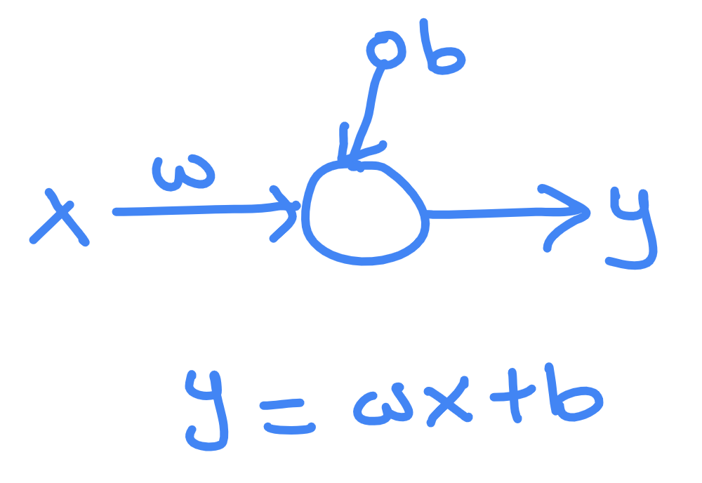
The visualization of the above neural network is as follows:

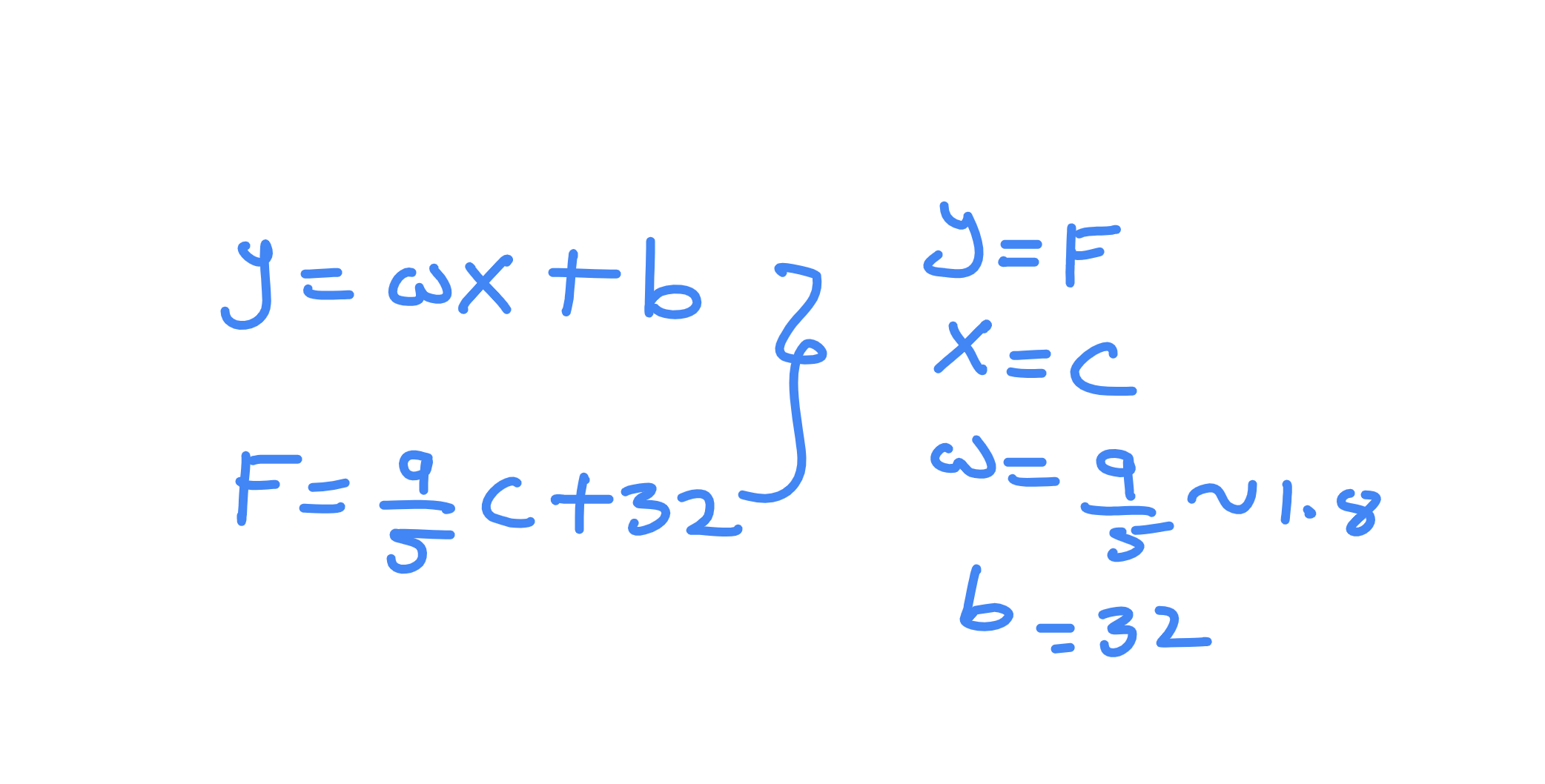
The equation of the above neural network can be compared to that of the equation of the celcius to farenheit as follows:  

Once we have our neural network initialized, let’s configure our model for training. The compile method of the Model class is responsible for defining loss function, optimizer (ADAM in our case), and metrics:

model.compile(

    loss='mean_squared_error', 

    optimizer=tf.keras.optimizers.Adam(0.1)

)

We have data and neural network setup, now we’ll train the model using the fit method with 500 epochs. The Epochs defines the number of times our model is going to be trained on the training dataset. 

model.fit(X, y, epochs=500, verbose=False)

After training the model we’ll infer from new data:

print(model.predict([98, 55]))

Output:

[[208.14742]

 [130.82669]]

Now, let’s check the weights of the neural network by using the get_weights() method as follows:

print(model.get_weights())

Output:

[array([[1.7981565]], dtype=float32), array([31.928087], dtype=float32)]

As you can see from the above result, the weight and bias of the trained model is closer to the value of the celsius to fahrenheit formula. The weight is 1.7981565, and bias is 31.928087 which is closer to 1.8 and 32 respectively.

This blog post should familiarize you with the very basics of writing ML programs and understanding what goes behind the scenes of learning the model.

• Recently Posted Data Scientist Jobs

• High Paying Marketing Jobs

• Part Time Software Developer Jobs

• Part Time Web Designer Jobs

• Top Paying Computer Programmer Jobs

• Top Paying Financial Manager Jobs